Josh's Blog | Optimal betting when odds are random

Optimal betting when odds are random

Since 1956, much has been written about optimal betting strategies for a gambler who is faced with an infinite sequence of profitable bets. Here I will briefly describe the “Kelly criterion” for optimal bet sizes and extend the discussion to situations where the odds attached to winning are a random variable. Finally I will discuss the these results in the context of betting in financial markets.

An even-odds bet where the probability of winning is greater than $50\%$ is an example of a profitable bet. How much should you wager, as a fraction of your capital, given the opportunity to place this bet infinitely many times in a row? In 1956 J. L. Kelly Jr., a researcher at Bell Labs, solved the question with the goal of maximizing the growth rate of capital. In the situation with even odds, to maximize the growth rate you should bet the fraction $f=p - q$ of your wealth, where $p$ is the probability of winning and $q = 1 – p$ is the probability of losing. For instance if you gain your bet with probability $p = 75\%$ and lose your bet with probability $q = 25\%$, then you should wager $50\%$ of your capital in each period in order to maximize its growth rate over the long term. As has been well-documented, betting “full Kelly” is quite aggressive and can lead to large losses over the short term. In this case there is a $25\%$ chance of losing half of one's wealth in a single bet! It is not for everybody, but from the perspective of wealth generation it dominates any other strategy over time.

Fixed odds

What fraction $f$ should we wager when the bets pay odds $b$ not necessarily equal to 1? Kelly's insight is that we can find the growth-rate-optimal betting fraction $f^*$ by maximizing our expected log of wealth in a single period. Without loss of generality we can normalize our current wealth to be 1, in which case $f^*$ maximizes

$$E\{\log_{}(\text{wealth})\}=p\log_{}(1+bf)+q\log_{}(1-f)$$

Taking the derivative with respect to $f$, setting equal to zero, and examining second derivative properties gives a maximum at

$$f^*=\frac{pb-q}{b}$$

Thus, $f^*$ is the “edge” divided by the odds. Notice that for an even odds bet, $b=1$ and $f^*=p – q$ as stated above.

Random odds

Case #1: discrete uniform

Let’s now consider adding a random component to the odds $b$. We may still lose our entire bet $f$ with probability $q$, but instead of winning $bf$ with probability $p$, we win

\begin{align} (b-\alpha)f \text{ with probability }0.5p \\ (b+\alpha)f \text{ with probability }0.5p \end{align}

for some $\alpha \geq 0$. The odds are still $b$ in expectation, but if $\alpha > 0$ then there is some variation thrown in the mix. By the concavity of the $\log$ function (Jensen's inequality), we will want to bet somewhat less than the optimal bet amount in the fixed-odds case, which I label $f^*_{\alpha=0}$.

What actually is the optimal fraction to bet? How does it relate to $f^*_{\alpha=0}$?

Let's define a discrete uniform random variable $X$ with the following distribution:

\begin{equation} X = \begin{cases} b-\alpha & \text{with probability $0.5$} \\ b+\alpha & \text{with probability $0.5$} \end{cases} \end{equation}

$$E(X)=b$$

$$Var(X)=E(X^2)-E(X)^2=\alpha^2$$

We want to maximize

\begin{align} E\{\log_{}(\text{wealth})\}&=E\{p\log_{}(1+Xf)+q\log_{}(1-f)\} \\ & = 0.5p\log_{}(1+(b-\alpha)f)+0.5p\log_{}(1+(b+\alpha)f)+q\log_{}(1-f) \end{align}

To maximize this we again take the derivative with respect to $f$ and set it to zero. Some algebra yields the quadratic equation

$$0=-(b^2–a^2)f^2 + (p(b^2–a^2) + b(p–2))f + p(b+1) – 1$$

Let’s examine this in the case where $\alpha=b$. The solution to the equation then becomes

$$\begin{eqnarray} f^*=\frac{pb-q}{b(1+q)}=\frac{f^*_{\alpha=0}}{1+q} \end{eqnarray}$$

With $q>0$, the optimal bet size is the fixed-odds optimal bet size multiplied by a factor less than 1. In the betting setup first described in the previous section, with even odds and $p=75\%$, the growth rate optimal bet amount is reduced from $50\%$ to $40\%$ when $\alpha=1$.

To keep things simple let’s stick with the even-odds case for the remainder of this post. Setting $b = 1$ into the quadratic equation turns it into

$$0 = -vf^2 + (p(v+1) - 2)f + 2p – 1 \text{ where }v = (1 - \alpha^2)$$

For $\alpha^2=Var(X)\ne 1$, the solution becomes:

$$f^*=\frac{2-p(v+1)\pm\sqrt{p^2(v+1)^2+4(p-1)(v-1)}}{-2v}$$

We can quickly check which of the two roots to use by setting $\alpha^2=0 \Rightarrow v=1$, in which case we have removed the random component and are back to the fixed-odds scenario. The minus sign gives the anticipated result $f^*=f^*_{\alpha=0, \text{ }b=1}=p-q$.

Case #2: continuous uniform

What if our random odds are continuous and distributed uniformly over the entire interval $[b-\alpha, b+\alpha]$?

Let $Y$ denote these new random odds, with probability density function

\begin{equation} g_Y(y) = \begin{cases} \frac{1}{2\alpha} & y \in [b-\alpha, b+\alpha] \\ 0 & \text{otherwise} \end{cases} \end{equation}

Note that

$$Var(Y)=\frac{4}{12}\alpha^2=\frac{1}{3}Var(X) < Var(X) \text{ when } \alpha>0$$

so that we should be betting more than the discrete-odds case of the previous section for any $\alpha>0$. It can be shown that $X$ has the highest possible variance of any random variable over the interval $[b-\alpha, b+\alpha]$, a fact which we will use in the next section to generate conservative betting estimates.

Now our objective function is

\begin{align} E\{\log_{}(\text{wealth})\}&=E\{p\log_{}(1+Yf)+q\log_{}(1-f)\} \\ & = \int_{b-\alpha}^{b+\alpha} \! p\log(1+yf) \, g_Y(y)\mathrm{d}y + q\log(1-f) \\ & = \frac{p}{2\alpha}\int_{b-\alpha}^{b+\alpha} \! \log(1+yf) \, \mathrm{d}y + q\log(1-f) \end{align}

Which we maximize by taking the derivative with respect to $f$ and setting equal to zero

\begin{align} 0 &= \frac{p}{2{\alpha}} \int_{b-\alpha}^{b+\alpha} \! \frac{y}{1+fy}\mathrm{d}y - \frac{q}{1-f} \\ &= \frac{p}{2{\alpha}f} \int_{b-\alpha}^{b+\alpha} \! \frac{fy}{1+fy}\mathrm{d}y - \frac{q}{1-f} \\ &= \frac{p}{2{\alpha}f} \left( \int_{b-\alpha}^{b+\alpha} \! \mathrm{d}y - \int_{b-\alpha}^{b+\alpha} \! \frac{\mathrm{d}y}{1+fy} \right) - \frac{q}{1-f} \\ &= \frac{p}{2{\alpha}f} \left( 2\alpha - \frac{1}{f}\log\left(\frac{1+(b+\alpha)f}{1+(b-\alpha)f}\right) \right) - \frac{q}{1-f} \end{align}

Solving numerically for the even-expected-odds case $(b=1)$ for various $p$ and $\alpha$ gives the following plot for $f^*$. Also included is the same plot for the discrete random odds case.

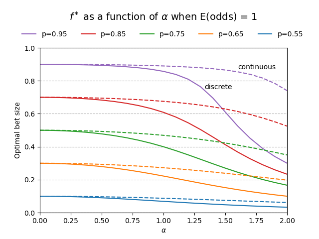
Notice that as $\alpha \to 0$ the optimal bet amounts converge to the corresponding fixed-odds optimal bet amounts. In the case of $p=75\%$, we can see from the chart that the optimal amount to bet is $50\%$ with fixed odds, and following the solid green line to $\alpha=1.00$, the optimal bet amount in the discrete random odds case is $40\%$, which we proved mathematically in the previous section. Some final things to notice are that $f^{*}$ in the case of continuously-distributed random odds is greater than the corresponding $f^*$ for discrete random odds when $\alpha > 0$, and even though the difference is not much for $\alpha$ near zero, it can be considerable for larger $\alpha$.

Application to financial markets

Below is an example of a potential scenario in which the above results may be helpful. But it does not constitute financial advice, and you should not trade options unless you are experienced.

A not-illegal rumor is swirling that company XYZ will receive an acquisition offer some time before the third Friday of the month. Relevant details are:

XYZ stock trades for €100
You assign $p=25\%$ to the probability of there being a legitimate offer in this time frame
Should an offer come, you expect it to be for €130 per share, but may be as low as €120 or as high as €140
Call options on XYZ with strike of €120 cost €1
If an offer is made, XYZ stock will jump to the offer price, otherwise it will languish and the option will expire worthless

Assuming your portfolio is all cash and that this XYZ option is the only investible game in town, what fraction might you want to bet on the XYZ €120 call?

Given the option costs €1, the realized odds of this bet in the event of an offer will range from -1 at €120 to +19 at €140. This corresponds to a random odds scenario as described in the post, with $p=25\%, b=9, \text{and } \alpha=10$. We can use the results above to calculate the bet amounts.

With the ability to make this investment infinitely many times (!), the growth-rate optimal bet amounts are:

16.67% if you fully believe that the offer will be €130 and nothing else (this is the $\alpha=0$ fixed odds case)
13.78% if you believe that the offer has an equal chance of being any price between €120 and €140 (uniform continuous odds case)
7.89% if you want to be conservative (uniform discrete odds case)

Conclusion

This post started with an explanation of classic growth-rate-optimal (Kelly) betting with odds $b$, and extended the idea to two cases in which odds are a random variable with expected value $b$ over a fixed interval.

The length of the interval is linked to the variance of the odds and inversely to the growth-rate optimal bet amount $f^*$.

For large $\alpha$ relative to $b$, $f^*$ can vary greatly depending on how the odds are actually distributed, something which can be seen in the plot and in the application to options trading in the final section.

posted at 00:00